As some of you may know, I spend 3 hours a day on the train travelling from cow country in Regional Victoria to the big smoke Melbourne…what a perfect time to test the power of Excel formulas to the limits. Now some of you may think Excel is just for managers crunching financial numbers…actually although I do use Excel quite a bit, I’m maybe one of those rare people who almost never uses it for financial information (ok except budgeting for my next high-end PC build)
So to start with I have a list of some IP addresses and their subnet address such as below:
Now I want to group them by network address…to do this we must check the IP address against the subnet. So there are a few stages we’re going to have to go through:
1) Split up the numbers by the decimal point
2) Convert each section to binary
3) Join the sections into one big binary number
4) Take the 1s from IP Address when there is a 1 in the SUBNET , other wise get 0s
5) Split binary number into 4 parts of 8
6) Convert back to decimal
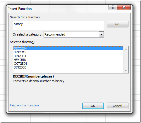
Seems a bit complicated for Excel, eh? But not at all, especially if you have 3 hrs on a train to kill. Because my memory is constantly being replaced with new technology I couldn’t think off the top of my head what formulas I’d use, so I started with the fx icon
So I used this to get the first part of the IP address (Small steps at a time)
=MID(A2,1,FIND(“.”,A2,1)-1)
To get the second value in the IP address the formula gets more complex.
=MID(A2,FIND(“.”,A2)+1,FIND(“.”,A2,(FIND(“.”,A2)+1)-FIND(“.”,A2))-1)
and for the 3rd IP octect:
=MID(A2,FIND(“.”,A2,FIND(“.”,A2)+1)+1,FIND(“.”,A2,FIND(“.”,A2,FIND(“.”,A2)+1)+1)-FIND(“.”,A2,FIND(“.”,A2)+1)-1)
At this point I strongly recommend a double-shot espresso to prevent brain disintegration before continuing.
Now for the fourth and final octet:
=MID(A2,FIND(“.”,A2,FIND(“.”,A2,FIND(“.”,A2)+1)+1)+1,LEN(A2)-FIND(“.”,A2,FIND(“.”,A2,FIND(“.”,A2)+1)+1)+1)
Now that’s the easy part, right? Well now we have to convert the four components into binary…How can we do this…again we go to our “fx” lookup and type in “binary” and click GO. Well pretty sweet – we can see Dec2Bin, a function is already there for us!
So use CONCATENATE to combine all binary numbers into one big mother binary number:
OK i’ll admit my first attempt didn’t work
After some corrections it started working:
=CONCATENATE(DEC2BIN(MID(A2,1,FIND(“.”,A2,1)-1),8),DEC2BIN(MID(A2,FIND(“.”,A2)+1,FIND(“.”,A2,(FIND(“.”,A2)+1)-FIND(“.”,A2))-1),8),DEC2BIN(MID(A2,FIND(“.”,A2,FIND(“.”,A2)+1)+1,FIND(“.”,A2,FIND(“.”,A2,FIND(“.”,A2)+1)+1)-FIND(“.”,A2,FIND(“.”,A2)+1)-1),8),DEC2BIN(MID(A2,FIND(“.”,A2,FIND(“.”,A2,FIND(“.”,A2)+1)+1)+1,LEN(A2)-FIND(“.”,A2,FIND(“.”,A2,FIND(“.”,A2)+1)+1)+1),8))
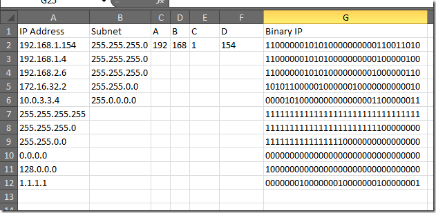
I did some test IP addresses to make sure it’s working
OK looks accurate…now for the final part we have to figure out how we do our subnet math…I dragged the formula across to the right to automatically get our subnets in binary
=CONCATENATE(DEC2BIN(MID(B2,1,FIND(“.”,B2,1)-1),8),DEC2BIN(MID(B2,FIND(“.”,B2)+1,FIND(“.”,B2,(FIND(“.”,B2)+1)-FIND(“.”,B2))-1),8),DEC2BIN(MID(B2,FIND(“.”,B2,FIND(“.”,B2)+1)+1,FIND(“.”,B2,FIND(“.”,B2,FIND(“.”,B2)+1)+1)-FIND(“.”,B2,FIND(“.”,B2)+1)-1),8),DEC2BIN(MID(B2,FIND(“.”,B2,FIND(“.”,B2,FIND(“.”,B2)+1)+1)+1,LEN(B2)-FIND(“.”,B2,FIND(“.”,B2,FIND(“.”,B2)+1)+1)+1),8))
So we then look for the position of ‘first’ 0 in the binary subnet –> we then extract everything from the binary IP up to that first zero. Maybe it’s not fool proof if you have some really funky subnets that are not all 1s followed by all 0s, but if we did a more precise formula, the formula would be REALLY massive, making this one look tiny.
=CONCATENATE(MID(G2,1,FIND(“0”,H2)-1),MID(H2,FIND(“0”,H2),33-FIND(“0”,H2)))
Now I’m quite happy to have the network address and leave it in binary, it looks pretty nice, and all the bits are really clear. But for those of you who grew up on decimal, here is what we do to get it back to a decimal address:
=CONCATENATE(BIN2DEC(MID(I2,1,8)),”.”,BIN2DEC(MID(I2,9,8)),”.”,BIN2DEC(MID(I2,17,8)),”.”,BIN2DEC(MID(I2,26,8)))
OK so now we’ve got our Network address in binary, as you can see in column J.
The final process is to combine all the formulas into one big formula…this is not going to work really well in excel’s formula editor, so I’m going to use notepad. I start by copying the formula in J2 and pasting it into Notepad. Then I’ll copy the formula from I2 and do a search replace on all instances of I2 to the formula in I2. This gets repeated down the line…i.e. replace H2 with formula in H2, replace G2 with formula in G2, etc.
But as my formula got bigger, notepad couldn’t handle the size of my search & replaces…so I went to my other editor…PSPad…
The formula is pretty massive, 7,720 characters long to be exact. But it WORKS!!!!
Here it is in all it’s glory…
=CONCATENATE(BIN2DEC(MID(CONCATENATE(MID(CONCATENATE(DEC2BIN(MID(A2,1,FIND(“.”,A2,1)-1),8),DEC2BIN(MID(A2,FIND(“.”,A2)+1,FIND(“.”,A2,(FIND(“.”,A2)+1)-FIND(“.”,A2))-1),8),DEC2BIN(MID(A2,FIND(“.”,A2,FIND(“.”,A2)+1)+1,FIND(“.”,A2,FIND(“.”,A2,FIND(“.”,A2)+1)+1)-FIND(“.”,A2,FIND(“.”,A2)+1)-1),8),DEC2BIN(MID(A2,FIND(“.”,A2,FIND(“.”,A2,FIND(“.”,A2)+1)+1)+1,LEN(A2)-FIND(“.”,A2,FIND(“.”,A2,FIND(“.”,A2)+1)+1)+1),8)),1,FIND(“0”,CONCATENATE(DEC2BIN(MID(B2,1,FIND(“.”,B2,1)-1),8),DEC2BIN(MID(B2,FIND(“.”,B2)+1,FIND(“.”,B2,(FIND(“.”,B2)+1)-FIND(“.”,B2))-1),8),DEC2BIN(MID(B2,FIND(“.”,B2,FIND(“.”,B2)+1)+1,FIND(“.”,B2,FIND(“.”,B2,FIND(“.”,B2)+1)+1)-FIND(“.”,B2,FIND(“.”,B2)+1)-1),8),DEC2BIN(MID(B2,FIND(“.”,B2,FIND(“.”,B2,FIND(“.”,B2)+1)+1)+1,LEN(B2)-FIND(“.”,B2,FIND(“.”,B2,FIND(“.”,B2)+1)+1)+1),8)))-1),MID(CONCATENATE(DEC2BIN(MID(B2,1,FIND(“.”,B2,1)-1),8),DEC2BIN(MID(B2,FIND(“.”,B2)+1,FIND(“.”,B2,(FIND(“.”,B2)+1)-FIND(“.”,B2))-1),8),DEC2BIN(MID(B2,FIND(“.”,B2,FIND(“.”,B2)+1)+1,FIND(“.”,B2,FIND(“.”,B2,FIND(“.”,B2)+1)+1)-FIND(“.”,B2,FIND(“.”,B2)+1)-1),8),DEC2BIN(MID(B2,FIND(“.”,B2,FIND(“.”,B2,FIND(“.”,B2)+1)+1)+1,LEN(B2)-FIND(“.”,B2,FIND(“.”,B2,FIND(“.”,B2)+1)+1)+1),8)),FIND(“0”,CONCATENATE(DEC2BIN(MID(B2,1,FIND(“.”,B2,1)-1),8),DEC2BIN(MID(B2,FIND(“.”,B2)+1,FIND(“.”,B2,(FIND(“.”,B2)+1)-FIND(“.”,B2))-1),8),DEC2BIN(MID(B2,FIND(“.”,B2,FIND(“.”,B2)+1)+1,FIND(“.”,B2,FIND(“.”,B2,FIND(“.”,B2)+1)+1)-FIND(“.”,B2,FIND(“.”,B2)+1)-1),8),DEC2BIN(MID(B2,FIND(“.”,B2,FIND(“.”,B2,FIND(“.”,B2)+1)+1)+1,LEN(B2)-FIND(“.”,B2,FIND(“.”,B2,FIND(“.”,B2)+1)+1)+1),8))),33-FIND(“0”,CONCATENATE(DEC2BIN(MID(B2,1,FIND(“.”,B2,1)-1),8),DEC2BIN(MID(B2,FIND(“.”,B2)+1,FIND(“.”,B2,(FIND(“.”,B2)+1)-FIND(“.”,B2))-1),8),DEC2BIN(MID(B2,FIND(“.”,B2,FIND(“.”,B2)+1)+1,FIND(“.”,B2,FIND(“.”,B2,FIND(“.”,B2)+1)+1)-FIND(“.”,B2,FIND(“.”,B2)+1)-1),8),DEC2BIN(MID(B2,FIND(“.”,B2,FIND(“.”,B2,FIND(“.”,B2)+1)+1)+1,LEN(B2)-FIND(“.”,B2,FIND(“.”,B2,FIND(“.”,B2)+1)+1)+1),8))))),1,8)),”.”,BIN2DEC(MID(CONCATENATE(MID(CONCATENATE(DEC2BIN(MID(A2,1,FIND(“.”,A2,1)-1),8),DEC2BIN(MID(A2,FIND(“.”,A2)+1,FIND(“.”,A2,(FIND(“.”,A2)+1)-FIND(“.”,A2))-1),8),DEC2BIN(MID(A2,FIND(“.”,A2,FIND(“.”,A2)+1)+1,FIND(“.”,A2,FIND(“.”,A2,FIND(“.”,A2)+1)+1)-FIND(“.”,A2,FIND(“.”,A2)+1)-1),8),DEC2BIN(MID(A2,FIND(“.”,A2,FIND(“.”,A2,FIND(“.”,A2)+1)+1)+1,LEN(A2)-FIND(“.”,A2,FIND(“.”,A2,FIND(“.”,A2)+1)+1)+1),8)),1,FIND(“0”,CONCATENATE(DEC2BIN(MID(B2,1,FIND(“.”,B2,1)-1),8),DEC2BIN(MID(B2,FIND(“.”,B2)+1,FIND(“.”,B2,(FIND(“.”,B2)+1)-FIND(“.”,B2))-1),8),DEC2BIN(MID(B2,FIND(“.”,B2,FIND(“.”,B2)+1)+1,FIND(“.”,B2,FIND(“.”,B2,FIND(“.”,B2)+1)+1)-FIND(“.”,B2,FIND(“.”,B2)+1)-1),8),DEC2BIN(MID(B2,FIND(“.”,B2,FIND(“.”,B2,FIND(“.”,B2)+1)+1)+1,LEN(B2)-FIND(“.”,B2,FIND(“.”,B2,FIND(“.”,B2)+1)+1)+1),8)))-1),MID(CONCATENATE(DEC2BIN(MID(B2,1,FIND(“.”,B2,1)-1),8),DEC2BIN(MID(B2,FIND(“.”,B2)+1,FIND(“.”,B2,(FIND(“.”,B2)+1)-FIND(“.”,B2))-1),8),DEC2BIN(MID(B2,FIND(“.”,B2,FIND(“.”,B2)+1)+1,FIND(“.”,B2,FIND(“.”,B2,FIND(“.”,B2)+1)+1)-FIND(“.”,B2,FIND(“.”,B2)+1)-1),8),DEC2BIN(MID(B2,FIND(“.”,B2,FIND(“.”,B2,FIND(“.”,B2)+1)+1)+1,LEN(B2)-FIND(“.”,B2,FIND(“.”,B2,FIND(“.”,B2)+1)+1)+1),8)),FIND(“0”,CONCATENATE(DEC2BIN(MID(B2,1,FIND(“.”,B2,1)-1),8),DEC2BIN(MID(B2,FIND(“.”,B2)+1,FIND(“.”,B2,(FIND(“.”,B2)+1)-FIND(“.”,B2))-1),8),DEC2BIN(MID(B2,FIND(“.”,B2,FIND(“.”,B2)+1)+1,FIND(“.”,B2,FIND(“.”,B2,FIND(“.”,B2)+1)+1)-FIND(“.”,B2,FIND(“.”,B2)+1)-1),8),DEC2BIN(MID(B2,FIND(“.”,B2,FIND(“.”,B2,FIND(“.”,B2)+1)+1)+1,LEN(B2)-FIND(“.”,B2,FIND(“.”,B2,FIND(“.”,B2)+1)+1)+1),8))),33-FIND(“0”,CONCATENATE(DEC2BIN(MID(B2,1,FIND(“.”,B2,1)-1),8),DEC2BIN(MID(B2,FIND(“.”,B2)+1,FIND(“.”,B2,(FIND(“.”,B2)+1)-FIND(“.”,B2))-1),8),DEC2BIN(MID(B2,FIND(“.”,B2,FIND(“.”,B2)+1)+1,FIND(“.”,B2,FIND(“.”,B2,FIND(“.”,B2)+1)+1)-FIND(“.”,B2,FIND(“.”,B2)+1)-1),8),DEC2BIN(MID(B2,FIND(“.”,B2,FIND(“.”,B2,FIND(“.”,B2)+1)+1)+1,LEN(B2)-FIND(“.”,B2,FIND(“.”,B2,FIND(“.”,B2)+1)+1)+1),8))))),9,8)),”.”,BIN2DEC(MID(CONCATENATE(MID(CONCATENATE(DEC2BIN(MID(A2,1,FIND(“.”,A2,1)-1),8),DEC2BIN(MID(A2,FIND(“.”,A2)+1,FIND(“.”,A2,(FIND(“.”,A2)+1)-FIND(“.”,A2))-1),8),DEC2BIN(MID(A2,FIND(“.”,A2,FIND(“.”,A2)+1)+1,FIND(“.”,A2,FIND(“.”,A2,FIND(“.”,A2)+1)+1)-FIND(“.”,A2,FIND(“.”,A2)+1)-1),8),DEC2BIN(MID(A2,FIND(“.”,A2,FIND(“.”,A2,FIND(“.”,A2)+1)+1)+1,LEN(A2)-FIND(“.”,A2,FIND(“.”,A2,FIND(“.”,A2)+1)+1)+1),8)),1,FIND(“0”,CONCATENATE(DEC2BIN(MID(B2,1,FIND(“.”,B2,1)-1),8),DEC2BIN(MID(B2,FIND(“.”,B2)+1,FIND(“.”,B2,(FIND(“.”,B2)+1)-FIND(“.”,B2))-1),8),DEC2BIN(MID(B2,FIND(“.”,B2,FIND(“.”,B2)+1)+1,FIND(“.”,B2,FIND(“.”,B2,FIND(“.”,B2)+1)+1)-FIND(“.”,B2,FIND(“.”,B2)+1)-1),8),DEC2BIN(MID(B2,FIND(“.”,B2,FIND(“.”,B2,FIND(“.”,B2)+1)+1)+1,LEN(B2)-FIND(“.”,B2,FIND(“.”,B2,FIND(“.”,B2)+1)+1)+1),8)))-1),MID(CONCATENATE(DEC2BIN(MID(B2,1,FIND(“.”,B2,1)-1),8),DEC2BIN(MID(B2,FIND(“.”,B2)+1,FIND(“.”,B2,(FIND(“.”,B2)+1)-FIND(“.”,B2))-1),8),DEC2BIN(MID(B2,FIND(“.”,B2,FIND(“.”,B2)+1)+1,FIND(“.”,B2,FIND(“.”,B2,FIND(“.”,B2)+1)+1)-FIND(“.”,B2,FIND(“.”,B2)+1)-1),8),DEC2BIN(MID(B2,FIND(“.”,B2,FIND(“.”,B2,FIND(“.”,B2)+1)+1)+1,LEN(B2)-FIND(“.”,B2,FIND(“.”,B2,FIND(“.”,B2)+1)+1)+1),8)),FIND(“0”,CONCATENATE(DEC2BIN(MID(B2,1,FIND(“.”,B2,1)-1),8),DEC2BIN(MID(B2,FIND(“.”,B2)+1,FIND(“.”,B2,(FIND(“.”,B2)+1)-FIND(“.”,B2))-1),8),DEC2BIN(MID(B2,FIND(“.”,B2,FIND(“.”,B2)+1)+1,FIND(“.”,B2,FIND(“.”,B2,FIND(“.”,B2)+1)+1)-FIND(“.”,B2,FIND(“.”,B2)+1)-1),8),DEC2BIN(MID(B2,FIND(“.”,B2,FIND(“.”,B2,FIND(“.”,B2)+1)+1)+1,LEN(B2)-FIND(“.”,B2,FIND(“.”,B2,FIND(“.”,B2)+1)+1)+1),8))),33-FIND(“0”,CONCATENATE(DEC2BIN(MID(B2,1,FIND(“.”,B2,1)-1),8),DEC2BIN(MID(B2,FIND(“.”,B2)+1,FIND(“.”,B2,(FIND(“.”,B2)+1)-FIND(“.”,B2))-1),8),DEC2BIN(MID(B2,FIND(“.”,B2,FIND(“.”,B2)+1)+1,FIND(“.”,B2,FIND(“.”,B2,FIND(“.”,B2)+1)+1)-FIND(“.”,B2,FIND(“.”,B2)+1)-1),8),DEC2BIN(MID(B2,FIND(“.”,B2,FIND(“.”,B2,FIND(“.”,B2)+1)+1)+1,LEN(B2)-FIND(“.”,B2,FIND(“.”,B2,FIND(“.”,B2)+1)+1)+1),8))))),17,8)),”.”,BIN2DEC(MID(CONCATENATE(MID(CONCATENATE(DEC2BIN(MID(A2,1,FIND(“.”,A2,1)-1),8),DEC2BIN(MID(A2,FIND(“.”,A2)+1,FIND(“.”,A2,(FIND(“.”,A2)+1)-FIND(“.”,A2))-1),8),DEC2BIN(MID(A2,FIND(“.”,A2,FIND(“.”,A2)+1)+1,FIND(“.”,A2,FIND(“.”,A2,FIND(“.”,A2)+1)+1)-FIND(“.”,A2,FIND(“.”,A2)+1)-1),8),DEC2BIN(MID(A2,FIND(“.”,A2,FIND(“.”,A2,FIND(“.”,A2)+1)+1)+1,LEN(A2)-FIND(“.”,A2,FIND(“.”,A2,FIND(“.”,A2)+1)+1)+1),8)),1,FIND(“0”,CONCATENATE(DEC2BIN(MID(B2,1,FIND(“.”,B2,1)-1),8),DEC2BIN(MID(B2,FIND(“.”,B2)+1,FIND(“.”,B2,(FIND(“.”,B2)+1)-FIND(“.”,B2))-1),8),DEC2BIN(MID(B2,FIND(“.”,B2,FIND(“.”,B2)+1)+1,FIND(“.”,B2,FIND(“.”,B2,FIND(“.”,B2)+1)+1)-FIND(“.”,B2,FIND(“.”,B2)+1)-1),8),DEC2BIN(MID(B2,FIND(“.”,B2,FIND(“.”,B2,FIND(“.”,B2)+1)+1)+1,LEN(B2)-FIND(“.”,B2,FIND(“.”,B2,FIND(“.”,B2)+1)+1)+1),8)))-1),MID(CONCATENATE(DEC2BIN(MID(B2,1,FIND(“.”,B2,1)-1),8),DEC2BIN(MID(B2,FIND(“.”,B2)+1,FIND(“.”,B2,(FIND(“.”,B2)+1)-FIND(“.”,B2))-1),8),DEC2BIN(MID(B2,FIND(“.”,B2,FIND(“.”,B2)+1)+1,FIND(“.”,B2,FIND(“.”,B2,FIND(“.”,B2)+1)+1)-FIND(“.”,B2,FIND(“.”,B2)+1)-1),8),DEC2BIN(MID(B2,FIND(“.”,B2,FIND(“.”,B2,FIND(“.”,B2)+1)+1)+1,LEN(B2)-FIND(“.”,B2,FIND(“.”,B2,FIND(“.”,B2)+1)+1)+1),8)),FIND(“0”,CONCATENATE(DEC2BIN(MID(B2,1,FIND(“.”,B2,1)-1),8),DEC2BIN(MID(B2,FIND(“.”,B2)+1,FIND(“.”,B2,(FIND(“.”,B2)+1)-FIND(“.”,B2))-1),8),DEC2BIN(MID(B2,FIND(“.”,B2,FIND(“.”,B2)+1)+1,FIND(“.”,B2,FIND(“.”,B2,FIND(“.”,B2)+1)+1)-FIND(“.”,B2,FIND(“.”,B2)+1)-1),8),DEC2BIN(MID(B2,FIND(“.”,B2,FIND(“.”,B2,FIND(“.”,B2)+1)+1)+1,LEN(B2)-FIND(“.”,B2,FIND(“.”,B2,FIND(“.”,B2)+1)+1)+1),8))),33-FIND(“0”,CONCATENATE(DEC2BIN(MID(B2,1,FIND(“.”,B2,1)-1),8),DEC2BIN(MID(B2,FIND(“.”,B2)+1,FIND(“.”,B2,(FIND(“.”,B2)+1)-FIND(“.”,B2))-1),8),DEC2BIN(MID(B2,FIND(“.”,B2,FIND(“.”,B2)+1)+1,FIND(“.”,B2,FIND(“.”,B2,FIND(“.”,B2)+1)+1)-FIND(“.”,B2,FIND(“.”,B2)+1)-1),8),DEC2BIN(MID(B2,FIND(“.”,B2,FIND(“.”,B2,FIND(“.”,B2)+1)+1)+1,LEN(B2)-FIND(“.”,B2,FIND(“.”,B2,FIND(“.”,B2)+1)+1)+1),8))))),26,8)))
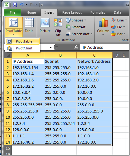
So now we can also create a Pivot table based on subnet…We can do this by selecting all cells by hitting Ctrl+A then selecting Insert tab and selecting PivotTable > PivotTable
Then range will already be selected, then click OK
In the PivotTable Field List we can drag Network Address into Values. We can sort by subnets with most PCs by clicking arrow on Row Labels and selecting More Sort Options > Descending (Z to A) by: Count of Network Address
In the PivotTable Field List we can now select what fields we want to be displayed, and they can be displayed in groups of subnets.
If you have any of your own “geeky” uses of Excel or a suggestion for a challenging Excel problem let me know ![]()
The .xlsx file used in this sample can be downloaded from here http://www.tiange.com.au/subnets.zip


Wow, this is very interesting and amazing, I think!
Just wondering – with the first part of splitting the IP address into column per octet – would using the Text to Columns function not be easier (using the “.” as the delimeter)?
Your function to trim my second octet isn’t working for me. My functions are in another language so, there could be missing there, but ok.
What I am wondering… you use in a formula: (FIND(“.”,A2)+1)-FIND(“.”,A2))
But this will allways give you the value 1, not?!
This is brilliant.
I do have one issue with the 2nd octet. It appears when I use 2 digits for the first octet i.e. 10.232.171.128 the second octet loses the last digit.
If I enter as 010.232.171.128 it appears to be working correctly, any suggestions as I have spent a few hours trying to work it out.
Many thanks.
Adam
Thank you very much. This helped me with getting my subnets from IP addresses for a report I had to do.
This was excellent. There is a minor error when the subnet mask is smaller than a Class C – is easily fixed, at the end of the forumla the number 26 needs to be changed to 25 – it was only evaluating the last 7 digits in the octet instead of 8.
yep that fixed it … this is really brilliant
There is a quicker more elegant way of breaking down an IP address into its parts by creating a custom function, see beow:
In excell open VBA (Macro -> Visual Basic Editor, or Ctrl+F11)
Insert -> Module
and, in that module type the text in-between the dashed lines:
——————————————————————————————————————
Public Function Octet(inIp As String, tetNo As Integer) as Byte
Dim a() As String
a = Split(inIp,”.”)
Octet = Cbyte(a(tetNo-1)) ‘ Subtract 1 for 1,2,3,4
End Function
——————————————————————————————————————
So for example if cell A3 has 192.168.1.129 and you enter the formula =Octet(A3,2) it will return the second octet or =Octet(A3,3) will return the 3rd octet etc…
You are cool man. Thank you.
Excellent work. You’re long train ride has saved me hours of work figuring out the same thing.
Nice, But how do you display the /24 bit from the valid IP Address?
if I put in 192.168.1.32 I would like to get 255.255.255.224 and a /27
in offce 2007 (transp view; )
IP-Address 4.69.17.254
Subnet Mask 255.255.255.248
addr_dot_1 =FIND(“.”;Table4[[#This row];[IP-Address]];1)
mask_dot_1 =FIND(“.”;Table4[[#This row];[Subnet Mask]];1)
addr_dot_2 =FIND(“.”;Table4[[#This row];[IP-Address]];Table4[[#This row];[addr_dot_1]]+1)
mask_dot_2 =FIND(“.”;Table4[[#This row];[Subnet Mask]];Table4[[#This row];[mask_dot_1]]+1)
addr_dot_3 =FIND(“.”;Table4[[#This row];[IP-Address]];Table4[[#This row];[addr_dot_2]]+1)
mask_dot_3 =FIND(“.”;Table4[[#This row];[Subnet Mask]];Table4[[#This row];[mask_dot_2]]+1)
addr_first =MID(Table4[[#This row];[IP-Address]];1;Table4[[#This row];[addr_dot_1]]-1)
mask_first =MID(Table4[[#This row];[Subnet Mask]];1;Table4[[#This row];[mask_dot_1]]-1)
addr_second =MID(Table4[[#This row];[IP-Address]];Table4[[#This row];[addr_dot_1]]+1;Table4[[#This row];[addr_dot_2]]-Table4[[#This row];[addr_dot_1]]-1)
mask_second =MID(Table4[[#This row];[Subnet Mask]];Table4[[#This row];[mask_dot_1]]+1;Table4[[#This row];[mask_dot_2]]-Table4[[#This row];[mask_dot_1]]-1)
addr_third =MID(Table4[[#This row];[IP-Address]];Table4[[#This row];[addr_dot_2]]+1;Table4[[#This row];[addr_dot_3]]-Table4[[#This row];[addr_dot_2]]-1)
mask_third =MID(Table4[[#This row];[Subnet Mask]];Table4[[#This row];[mask_dot_2]]+1;Table4[[#This row];[mask_dot_3]]-Table4[[#This row];[mask_dot_2]]-1)
addr_fourth =MID(Table4[[#This row];[IP-Address]];Table4[[#This row];[addr_dot_3]]+1;LEN(Table4[[#This row];[IP-Address]])-Table4[[#This row];[addr_dot_3]])
mask_fourth =MID(Table4[[#This row];[Subnet Mask]];Table4[[#This row];[mask_dot_3]]+1;LEN(Table4[[#This row];[Subnet Mask]])-Table4[[#This row];[mask_dot_3]])
addr_first2 =DEC2BIN(Table4[[#This row];[addr_first]];8)
mask_first3 =DEC2BIN(Table4[[#This row];[mask_first]];8)
addr_second4 =DEC2BIN(Table4[[#This row];[addr_second]];8)
mask_second5 =DEC2BIN(Table4[[#This row];[mask_second]];8)
addr_third6 =DEC2BIN(Table4[[#This row];[addr_third]];8)
mask_third7 =DEC2BIN(Table4[[#This row];[mask_third]];8)
addr_fourth8 =DEC2BIN(Table4[[#This row];[addr_fourth]];8)
mask_fourth9 =DEC2BIN(Table4[[#This row];[mask_fourth]];8)
addr_bin_concatenate =CONCATENATE(Table4[[#This row];[addr_first2]];Table4[[#This row];[addr_second4]];Table4[[#This row];[addr_third6]];Table4[[#This row];[addr_fourth8]])
mask_bin_concatenate =CONCATENATE(Table4[[#This row];[mask_first3]];Table4[[#This row];[mask_second5]];Table4[[#This row];[mask_third7]];Table4[[#This row];[mask_fourth9]])
0_pos_in_mask =FIND(0;Table4[[#This row];[mask_bin_concatenate]];1)
network_bin_arrd_part =LEFT(Table4[[#This row];[addr_bin_concatenate]];Table4[[#This row];[0_pos_in_mask]]-1)
network_bin_mask_part =RIGHT(Table4[[#This row];[mask_bin_concatenate]];33-Table4[[#This row];[0_pos_in_mask]])
network_bin_ =CONCATENATE(Table4[[#This row];[network_bin_arrd_part]];Table4[[#This row];[network_bin_mask_part]])
network_len =LEN(Table4[[#This row];[network_bin_]])
network_bin_1 =MID(Table4[[#This row];[network_bin_]];1;8)
network_bin_2 =MID(Table4[[#This row];[network_bin_]];9;8)
network_bin_3 =MID(Table4[[#This row];[network_bin_]];17;8)
network_bin_4 =MID(Table4[[#This row];[network_bin_]];25;32)
network_dec_1 =BIN2DEC(Table4[[#This row];[network_bin_1]])
network_dec_2 =BIN2DEC(Table4[[#This row];[network_bin_2]])
network_dec_3 =BIN2DEC(Table4[[#This row];[network_bin_3]])
network_dec_4 =BIN2DEC(Table4[[#This row];[network_bin_4]])
network_address =CONCATENATE(Table4[[#This row];[network_dec_1]];”.”;Table4[[#This row];[network_dec_2]];”.”;Table4[[#This row];[network_dec_3]];”.”;Table4[[#This row];[network_dec_4]])
Hi, just been reading through this and it looks great however I am having one or two problems with the formulas and I can’t seem to download it. Is it still available for download ?
I’ll try to upload somewhere else later
Am I not doing the things correctly or is there a bug in the second value in the IP address, if the first value has less that 3 digits??
there is a bug, fix in the comments(I think). I may not have uploaded the fix.
Hi chentiangemalc,
thank you very much for your quick answer.
Actually, I did not see Adam’s post, and did not see either your file (http://www.tiange.com.au/ gives a 404, BTW). I just copied/pasted the formulae I needed from your post.
FYI, I modified your formula for the second octet and used (where D2 is the full IP)
=IF(ISBLANK(D2),””,VALUE(LEFT(RIGHT(D2,LEN(D2)-FIND(“.”,D2)),FIND(“.”,RIGHT(D2,LEN(D2)-FIND(“.”,D2)))-1)))
(please check it as my Office suite is not in English, so the functions & syntax I use in Excel are not the same)
Regards
BS
I’m trying to get a subnet from entering a network address and a broadcast address. I can’t get it to work, but I’m trying to compare binary of the network address and the broadcast address to get the subnet mask. For example:
11000000101001110000000000000000 + 11000000101010001111111111111111 = 11111111111111100000000000000000
192.167..0.0 + 192.168.255.255 = 255.254.0.0
How do I configured Excel to do this? Thanks..
Actually, your example numbers don’t work. The 255.254.0.0 masked subnet that includes 192.168.255.255 goes from 192.168.0.0 to 192.169.255.255. The smallest subnet that includes 192.167.0.0 and 192.168.255.255 is 192.160.0.0/12 with a mask of 255.240.0.0 . You always have to be careful of CIDR boundaries when doing this stuff. Maybe your code was giving you the right answer and you didn’t realize it?
Hello,
Hope that you are doing fine.
I just have notice that last octet equation should be BIN2DEC(MID(I2,25,8)) not BIN2DEC(MID(I2,26,8)) in the formula where changing the network IP from binary to decimal.
Have a great day.
Yes that is correct. I thought I corrected this, but obviously not…
Your way for dividing the problem in steps is great…
I was trying to make formula like this but i was lazy as though that it would be hard to do.
Thank you for the great post, my problem is solved now :)
Hey man can you upload it somewhere else?
Thanks!
https://onedrive.live.com/redir?resid=E1A3C870740A073D!23010&authkey=!AKuKOKyhDNAw2YU&ithint=file%2cxlsb
Your formula only works if the second octate is the same size of the first one … 10.238.xxx.xxx for say a 255.255.xxx.xxx subnet gets chopped to 10.23. ..not 10.238
yes I fixed that but may not have uploaded the fix.
This is the most insane and insanely useful thing I’ve seen for a while. Thanks. I owe you beer.
You, sir, are a god among mortals! Thank you so much for this.
Of course, I have a question. I’m trying to munge the formulas so I can also find the first and last useable IP addresses in the range but I am being a monumental idiot and not able to do it.
If anyone has some help for me I’m sure it’s something many people would appreciate.
~W
Very good solution, save me time in working this all out. I also had an issue with the 2nd Octet giving 2 digit answers when it should have been 3. I removed a set of () from the formula
you have
=MID(A2,FIND(“.”,A2)+1,FIND(“.”,A2,(FIND(“.”,A2)+1)-FIND(“.”,A2))-1)
this worked for me
=MID(A2,FIND(“.”,A2)+1,FIND(“.”,A2,FIND(“.”,A2)+1)-FIND(“.”,A2)-1)
Hi,
Binary IP and Binary Address formül is not working. Can I help me!
Thanks,
=CONCATENATE(DEC2BIN(MID(B2,1,FIND(“.”,B2,1)-1),8),DEC2BIN(MID(B2,FIND(“.”,B2)+1,FIND(“.”,B2,(FIND(“.”,B2)+1)-FIND(“.”,B2))-1),8),DEC2BIN(MID(B2,FIND(“.”,B2,FIND(“.”,B2)+1)+1,FIND(“.”,B2,FIND(“.”,B2,FIND(“.”,B2)+1)+1)-FIND(“.”,B2,FIND(“.”,B2)+1)-1),8),DEC2BIN(MID(B2,FIND(“.”,B2,FIND(“.”,B2,FIND(“.”,B2)+1)+1)+1,LEN(B2)-FIND(“.”,B2,FIND(“.”,B2,FIND(“.”,B2)+1)+1)+1),8))
Amazing
thank you for the tutorial. it is very helpful. However the URL to download file doesn’t work.
As always from Chentiangemalc amazing tools. link to download worked with no problems https://onedrive.live.com/redir?resid=E1A3C870740A073D!23010&authkey=!AKuKOKyhDNAw2YU&ithint=file%2cxlsb
and the subnets I checked are coming correct, save me lots of time building changes.
I am looking for such a related excel that we can calculate the range of IP according to demand. For instance we have 50 host and able to find first and last one.
Thee was a problem with subnets in which the last octet of the VLAN was 128 or larger. Replacng the trailing “26” in the formula with “25” fixed it for me. Here’s the formula with this fix and the fix identified by Gary:
=CONCATENATE(BIN2DEC(MID(CONCATENATE(MID(CONCATENATE(DEC2BIN(MID(A1,1,FIND(“.”,A1,1)-1),8),DEC2BIN(MID(A1,FIND(“.”,A1)+1,FIND(“.”,A1,FIND(“.”,A1)+1)-FIND(“.”,A1)-1),8),DEC2BIN(MID(A1,FIND(“.”,A1,FIND(“.”,A1)+1)+1,FIND(“.”,A1,FIND(“.”,A1,FIND(“.”,A1)+1)+1)-FIND(“.”,A1,FIND(“.”,A1)+1)-1),8),DEC2BIN(MID(A1,FIND(“.”,A1,FIND(“.”,A1,FIND(“.”,A1)+1)+1)+1,LEN(A1)-FIND(“.”,A1,FIND(“.”,A1,FIND(“.”,A1)+1)+1)+1),8)),1,FIND(“0”,CONCATENATE(DEC2BIN(MID(B1,1,FIND(“.”,B1,1)-1),8),DEC2BIN(MID(B1,FIND(“.”,B1)+1,FIND(“.”,B1,(FIND(“.”,B1)+1)-FIND(“.”,B1))-1),8),DEC2BIN(MID(B1,FIND(“.”,B1,FIND(“.”,B1)+1)+1,FIND(“.”,B1,FIND(“.”,B1,FIND(“.”,B1)+1)+1)-FIND(“.”,B1,FIND(“.”,B1)+1)-1),8),DEC2BIN(MID(B1,FIND(“.”,B1,FIND(“.”,B1,FIND(“.”,B1)+1)+1)+1,LEN(B1)-FIND(“.”,B1,FIND(“.”,B1,FIND(“.”,B1)+1)+1)+1),8)))-1),MID(CONCATENATE(DEC2BIN(MID(B1,1,FIND(“.”,B1,1)-1),8),DEC2BIN(MID(B1,FIND(“.”,B1)+1,FIND(“.”,B1,(FIND(“.”,B1)+1)-FIND(“.”,B1))-1),8),DEC2BIN(MID(B1,FIND(“.”,B1,FIND(“.”,B1)+1)+1,FIND(“.”,B1,FIND(“.”,B1,FIND(“.”,B1)+1)+1)-FIND(“.”,B1,FIND(“.”,B1)+1)-1),8),DEC2BIN(MID(B1,FIND(“.”,B1,FIND(“.”,B1,FIND(“.”,B1)+1)+1)+1,LEN(B1)-FIND(“.”,B1,FIND(“.”,B1,FIND(“.”,B1)+1)+1)+1),8)),FIND(“0”,CONCATENATE(DEC2BIN(MID(B1,1,FIND(“.”,B1,1)-1),8),DEC2BIN(MID(B1,FIND(“.”,B1)+1,FIND(“.”,B1,(FIND(“.”,B1)+1)-FIND(“.”,B1))-1),8),DEC2BIN(MID(B1,FIND(“.”,B1,FIND(“.”,B1)+1)+1,FIND(“.”,B1,FIND(“.”,B1,FIND(“.”,B1)+1)+1)-FIND(“.”,B1,FIND(“.”,B1)+1)-1),8),DEC2BIN(MID(B1,FIND(“.”,B1,FIND(“.”,B1,FIND(“.”,B1)+1)+1)+1,LEN(B1)-FIND(“.”,B1,FIND(“.”,B1,FIND(“.”,B1)+1)+1)+1),8))),33-FIND(“0”,CONCATENATE(DEC2BIN(MID(B1,1,FIND(“.”,B1,1)-1),8),DEC2BIN(MID(B1,FIND(“.”,B1)+1,FIND(“.”,B1,(FIND(“.”,B1)+1)-FIND(“.”,B1))-1),8),DEC2BIN(MID(B1,FIND(“.”,B1,FIND(“.”,B1)+1)+1,FIND(“.”,B1,FIND(“.”,B1,FIND(“.”,B1)+1)+1)-FIND(“.”,B1,FIND(“.”,B1)+1)-1),8),DEC2BIN(MID(B1,FIND(“.”,B1,FIND(“.”,B1,FIND(“.”,B1)+1)+1)+1,LEN(B1)-FIND(“.”,B1,FIND(“.”,B1,FIND(“.”,B1)+1)+1)+1),8))))),1,8)),”.”,BIN2DEC(MID(CONCATENATE(MID(CONCATENATE(DEC2BIN(MID(A1,1,FIND(“.”,A1,1)-1),8),DEC2BIN(MID(A1,FIND(“.”,A1)+1,FIND(“.”,A1,FIND(“.”,A1)+1)-FIND(“.”,A1)-1),8),DEC2BIN(MID(A1,FIND(“.”,A1,FIND(“.”,A1)+1)+1,FIND(“.”,A1,FIND(“.”,A1,FIND(“.”,A1)+1)+1)-FIND(“.”,A1,FIND(“.”,A1)+1)-1),8),DEC2BIN(MID(A1,FIND(“.”,A1,FIND(“.”,A1,FIND(“.”,A1)+1)+1)+1,LEN(A1)-FIND(“.”,A1,FIND(“.”,A1,FIND(“.”,A1)+1)+1)+1),8)),1,FIND(“0”,CONCATENATE(DEC2BIN(MID(B1,1,FIND(“.”,B1,1)-1),8),DEC2BIN(MID(B1,FIND(“.”,B1)+1,FIND(“.”,B1,(FIND(“.”,B1)+1)-FIND(“.”,B1))-1),8),DEC2BIN(MID(B1,FIND(“.”,B1,FIND(“.”,B1)+1)+1,FIND(“.”,B1,FIND(“.”,B1,FIND(“.”,B1)+1)+1)-FIND(“.”,B1,FIND(“.”,B1)+1)-1),8),DEC2BIN(MID(B1,FIND(“.”,B1,FIND(“.”,B1,FIND(“.”,B1)+1)+1)+1,LEN(B1)-FIND(“.”,B1,FIND(“.”,B1,FIND(“.”,B1)+1)+1)+1),8)))-1),MID(CONCATENATE(DEC2BIN(MID(B1,1,FIND(“.”,B1,1)-1),8),DEC2BIN(MID(B1,FIND(“.”,B1)+1,FIND(“.”,B1,(FIND(“.”,B1)+1)-FIND(“.”,B1))-1),8),DEC2BIN(MID(B1,FIND(“.”,B1,FIND(“.”,B1)+1)+1,FIND(“.”,B1,FIND(“.”,B1,FIND(“.”,B1)+1)+1)-FIND(“.”,B1,FIND(“.”,B1)+1)-1),8),DEC2BIN(MID(B1,FIND(“.”,B1,FIND(“.”,B1,FIND(“.”,B1)+1)+1)+1,LEN(B1)-FIND(“.”,B1,FIND(“.”,B1,FIND(“.”,B1)+1)+1)+1),8)),FIND(“0”,CONCATENATE(DEC2BIN(MID(B1,1,FIND(“.”,B1,1)-1),8),DEC2BIN(MID(B1,FIND(“.”,B1)+1,FIND(“.”,B1,(FIND(“.”,B1)+1)-FIND(“.”,B1))-1),8),DEC2BIN(MID(B1,FIND(“.”,B1,FIND(“.”,B1)+1)+1,FIND(“.”,B1,FIND(“.”,B1,FIND(“.”,B1)+1)+1)-FIND(“.”,B1,FIND(“.”,B1)+1)-1),8),DEC2BIN(MID(B1,FIND(“.”,B1,FIND(“.”,B1,FIND(“.”,B1)+1)+1)+1,LEN(B1)-FIND(“.”,B1,FIND(“.”,B1,FIND(“.”,B1)+1)+1)+1),8))),33-FIND(“0”,CONCATENATE(DEC2BIN(MID(B1,1,FIND(“.”,B1,1)-1),8),DEC2BIN(MID(B1,FIND(“.”,B1)+1,FIND(“.”,B1,(FIND(“.”,B1)+1)-FIND(“.”,B1))-1),8),DEC2BIN(MID(B1,FIND(“.”,B1,FIND(“.”,B1)+1)+1,FIND(“.”,B1,FIND(“.”,B1,FIND(“.”,B1)+1)+1)-FIND(“.”,B1,FIND(“.”,B1)+1)-1),8),DEC2BIN(MID(B1,FIND(“.”,B1,FIND(“.”,B1,FIND(“.”,B1)+1)+1)+1,LEN(B1)-FIND(“.”,B1,FIND(“.”,B1,FIND(“.”,B1)+1)+1)+1),8))))),9,8)),”.”,BIN2DEC(MID(CONCATENATE(MID(CONCATENATE(DEC2BIN(MID(A1,1,FIND(“.”,A1,1)-1),8),DEC2BIN(MID(A1,FIND(“.”,A1)+1,FIND(“.”,A1,FIND(“.”,A1)+1)-FIND(“.”,A1)-1),8),DEC2BIN(MID(A1,FIND(“.”,A1,FIND(“.”,A1)+1)+1,FIND(“.”,A1,FIND(“.”,A1,FIND(“.”,A1)+1)+1)-FIND(“.”,A1,FIND(“.”,A1)+1)-1),8),DEC2BIN(MID(A1,FIND(“.”,A1,FIND(“.”,A1,FIND(“.”,A1)+1)+1)+1,LEN(A1)-FIND(“.”,A1,FIND(“.”,A1,FIND(“.”,A1)+1)+1)+1),8)),1,FIND(“0”,CONCATENATE(DEC2BIN(MID(B1,1,FIND(“.”,B1,1)-1),8),DEC2BIN(MID(B1,FIND(“.”,B1)+1,FIND(“.”,B1,(FIND(“.”,B1)+1)-FIND(“.”,B1))-1),8),DEC2BIN(MID(B1,FIND(“.”,B1,FIND(“.”,B1)+1)+1,FIND(“.”,B1,FIND(“.”,B1,FIND(“.”,B1)+1)+1)-FIND(“.”,B1,FIND(“.”,B1)+1)-1),8),DEC2BIN(MID(B1,FIND(“.”,B1,FIND(“.”,B1,FIND(“.”,B1)+1)+1)+1,LEN(B1)-FIND(“.”,B1,FIND(“.”,B1,FIND(“.”,B1)+1)+1)+1),8)))-1),MID(CONCATENATE(DEC2BIN(MID(B1,1,FIND(“.”,B1,1)-1),8),DEC2BIN(MID(B1,FIND(“.”,B1)+1,FIND(“.”,B1,(FIND(“.”,B1)+1)-FIND(“.”,B1))-1),8),DEC2BIN(MID(B1,FIND(“.”,B1,FIND(“.”,B1)+1)+1,FIND(“.”,B1,FIND(“.”,B1,FIND(“.”,B1)+1)+1)-FIND(“.”,B1,FIND(“.”,B1)+1)-1),8),DEC2BIN(MID(B1,FIND(“.”,B1,FIND(“.”,B1,FIND(“.”,B1)+1)+1)+1,LEN(B1)-FIND(“.”,B1,FIND(“.”,B1,FIND(“.”,B1)+1)+1)+1),8)),FIND(“0”,CONCATENATE(DEC2BIN(MID(B1,1,FIND(“.”,B1,1)-1),8),DEC2BIN(MID(B1,FIND(“.”,B1)+1,FIND(“.”,B1,(FIND(“.”,B1)+1)-FIND(“.”,B1))-1),8),DEC2BIN(MID(B1,FIND(“.”,B1,FIND(“.”,B1)+1)+1,FIND(“.”,B1,FIND(“.”,B1,FIND(“.”,B1)+1)+1)-FIND(“.”,B1,FIND(“.”,B1)+1)-1),8),DEC2BIN(MID(B1,FIND(“.”,B1,FIND(“.”,B1,FIND(“.”,B1)+1)+1)+1,LEN(B1)-FIND(“.”,B1,FIND(“.”,B1,FIND(“.”,B1)+1)+1)+1),8))),33-FIND(“0”,CONCATENATE(DEC2BIN(MID(B1,1,FIND(“.”,B1,1)-1),8),DEC2BIN(MID(B1,FIND(“.”,B1)+1,FIND(“.”,B1,(FIND(“.”,B1)+1)-FIND(“.”,B1))-1),8),DEC2BIN(MID(B1,FIND(“.”,B1,FIND(“.”,B1)+1)+1,FIND(“.”,B1,FIND(“.”,B1,FIND(“.”,B1)+1)+1)-FIND(“.”,B1,FIND(“.”,B1)+1)-1),8),DEC2BIN(MID(B1,FIND(“.”,B1,FIND(“.”,B1,FIND(“.”,B1)+1)+1)+1,LEN(B1)-FIND(“.”,B1,FIND(“.”,B1,FIND(“.”,B1)+1)+1)+1),8))))),17,8)),”.”,BIN2DEC(MID(CONCATENATE(MID(CONCATENATE(DEC2BIN(MID(A1,1,FIND(“.”,A1,1)-1),8),DEC2BIN(MID(A1,FIND(“.”,A1)+1,FIND(“.”,A1,FIND(“.”,A1)+1)-FIND(“.”,A1)-1),8),DEC2BIN(MID(A1,FIND(“.”,A1,FIND(“.”,A1)+1)+1,FIND(“.”,A1,FIND(“.”,A1,FIND(“.”,A1)+1)+1)-FIND(“.”,A1,FIND(“.”,A1)+1)-1),8),DEC2BIN(MID(A1,FIND(“.”,A1,FIND(“.”,A1,FIND(“.”,A1)+1)+1)+1,LEN(A1)-FIND(“.”,A1,FIND(“.”,A1,FIND(“.”,A1)+1)+1)+1),8)),1,FIND(“0”,CONCATENATE(DEC2BIN(MID(B1,1,FIND(“.”,B1,1)-1),8),DEC2BIN(MID(B1,FIND(“.”,B1)+1,FIND(“.”,B1,(FIND(“.”,B1)+1)-FIND(“.”,B1))-1),8),DEC2BIN(MID(B1,FIND(“.”,B1,FIND(“.”,B1)+1)+1,FIND(“.”,B1,FIND(“.”,B1,FIND(“.”,B1)+1)+1)-FIND(“.”,B1,FIND(“.”,B1)+1)-1),8),DEC2BIN(MID(B1,FIND(“.”,B1,FIND(“.”,B1,FIND(“.”,B1)+1)+1)+1,LEN(B1)-FIND(“.”,B1,FIND(“.”,B1,FIND(“.”,B1)+1)+1)+1),8)))-1),MID(CONCATENATE(DEC2BIN(MID(B1,1,FIND(“.”,B1,1)-1),8),DEC2BIN(MID(B1,FIND(“.”,B1)+1,FIND(“.”,B1,(FIND(“.”,B1)+1)-FIND(“.”,B1))-1),8),DEC2BIN(MID(B1,FIND(“.”,B1,FIND(“.”,B1)+1)+1,FIND(“.”,B1,FIND(“.”,B1,FIND(“.”,B1)+1)+1)-FIND(“.”,B1,FIND(“.”,B1)+1)-1),8),DEC2BIN(MID(B1,FIND(“.”,B1,FIND(“.”,B1,FIND(“.”,B1)+1)+1)+1,LEN(B1)-FIND(“.”,B1,FIND(“.”,B1,FIND(“.”,B1)+1)+1)+1),8)),FIND(“0”,CONCATENATE(DEC2BIN(MID(B1,1,FIND(“.”,B1,1)-1),8),DEC2BIN(MID(B1,FIND(“.”,B1)+1,FIND(“.”,B1,(FIND(“.”,B1)+1)-FIND(“.”,B1))-1),8),DEC2BIN(MID(B1,FIND(“.”,B1,FIND(“.”,B1)+1)+1,FIND(“.”,B1,FIND(“.”,B1,FIND(“.”,B1)+1)+1)-FIND(“.”,B1,FIND(“.”,B1)+1)-1),8),DEC2BIN(MID(B1,FIND(“.”,B1,FIND(“.”,B1,FIND(“.”,B1)+1)+1)+1,LEN(B1)-FIND(“.”,B1,FIND(“.”,B1,FIND(“.”,B1)+1)+1)+1),8))),33-FIND(“0”,CONCATENATE(DEC2BIN(MID(B1,1,FIND(“.”,B1,1)-1),8),DEC2BIN(MID(B1,FIND(“.”,B1)+1,FIND(“.”,B1,(FIND(“.”,B1)+1)-FIND(“.”,B1))-1),8),DEC2BIN(MID(B1,FIND(“.”,B1,FIND(“.”,B1)+1)+1,FIND(“.”,B1,FIND(“.”,B1,FIND(“.”,B1)+1)+1)-FIND(“.”,B1,FIND(“.”,B1)+1)-1),8),DEC2BIN(MID(B1,FIND(“.”,B1,FIND(“.”,B1,FIND(“.”,B1)+1)+1)+1,LEN(B1)-FIND(“.”,B1,FIND(“.”,B1,FIND(“.”,B1)+1)+1)+1),8))))),25,8)))
P.S.: You’ll still need to handle the replacement of the “fancy font matching quotes” in the formula with standard non-matching quotes that Excel expects, otherwise you’ll get a #NAME?
error. The web site input box replaces the standard quotes with “fancy font matching quotes” when posting to the web site.
Can someone please upload the latest excel sheet. Unable to download from https://onedrive.live.com/redir?resid=E1A3C870740A073D!23010&authkey=!AKuKOKyhDNAw2YU&ithint=file%2cxlsb
OK, first off awesome, and thanks. I really needed this for some work I am doing in an environment where I cannot use VB Scripts or Macros, this helped a lot. However, There is an error which I cannot figure out how to correct.
regarding the Network ID formula
=CONCATENATE(MID(AK1,1,FIND(“0”,AR1)-1),MID(AR1,FIND(“0”,AR1),33-FIND(“0”,AR1)))
This does not work for instance when you have an IP address for example 10.10.10.129/25, the correct return s/b 10.10.10.128 for the network ID, the formula returns 10.10.10.0.
So… did I miss something somewhere? I can post my entire spreadsheet if necessary.
Darren
Yes I think there are some errors in the formula; I fixed some them will have to check if I uploaded it. It’s not the easiest thing to troubleshoot. To work out bugs reasonably easily you need to check the results of each section of the formula. In retrospect I should have just used a comptuer program to generate the formula.
Very helpful I will pass this along to my peers. Thanks!
A huge thanks for this, now I’m able to validate 2 hosts are in the same network in google sheet :)
Pingback: Finding IPs covered by Subnets in an Excel document – uuug
To calculate the IP range, use the binary columns used above (columns G, H, I) – the beginning is the network part of the IP address then all zeros ending with a “1”. The ending is the network part of the IP address then all ones ending with a “0”.
Beginning IP range binary: =CONCATENATE(MID(G2,1,FIND(“0”,H2)-1),REPT(“0”,33-FIND(“0″,H2)),”1”)
Ending IP range binary: =CONCATENATE(MID(G2,1,FIND(“0”,H2)-1),REPT(“1”,33-FIND(“0″,H2)),”0”)
Then convert each of these columns to decimal using the formula above that starts with “But for those of you who grew up on decimal, here is what we do to get it back to a decimal address:”
Hey … Don’t have enough words to thanks. I really want to talk to you and say THANKS for this amazing work.
I love all the input here. I cannot access any google drive type of sites. can someone give me a standard link to download and use a spreadsheet or email to tkspam000@gmail.com ?